Solving Problems by Searching


In this article, we will see how a problem-solving agent can use search trees to look ahead and find a sequence of actions that will solve our problem.
This method works particularly well in environments that are deterministic, fully observable, static, discrete, and known. Search trees can be used to solve multi-agent environments, which we will discuss in another article. In this article, we will only cover single-agent environments. Also, search problems must have atomic states; states with no internal structure or components.
We will start by introducing systematic algorithms, also known as uninformed algorithms, and in the next article, we will move on to intelligent algorithms, also known as informed algorithms.
Problem-solving agents are currently used in many real-world situations. Path finding in video games, routing video streams in computer networks, and finding optimal driving directions are amongst the first examples that come to mind. Those are known as route-finding problems.
But they are also used for touring problems (travelling salesperson problem) where a salesman needs to travel to every city most efficiently, VLSI layout problems where millions of transistors need to be strategically placed on a single chip to minimize area and signal delay (propagation delay). They are even used in robot navigation and automatic assembly sequencing.
Search Problems
We will start with a simple route-finding search problem.
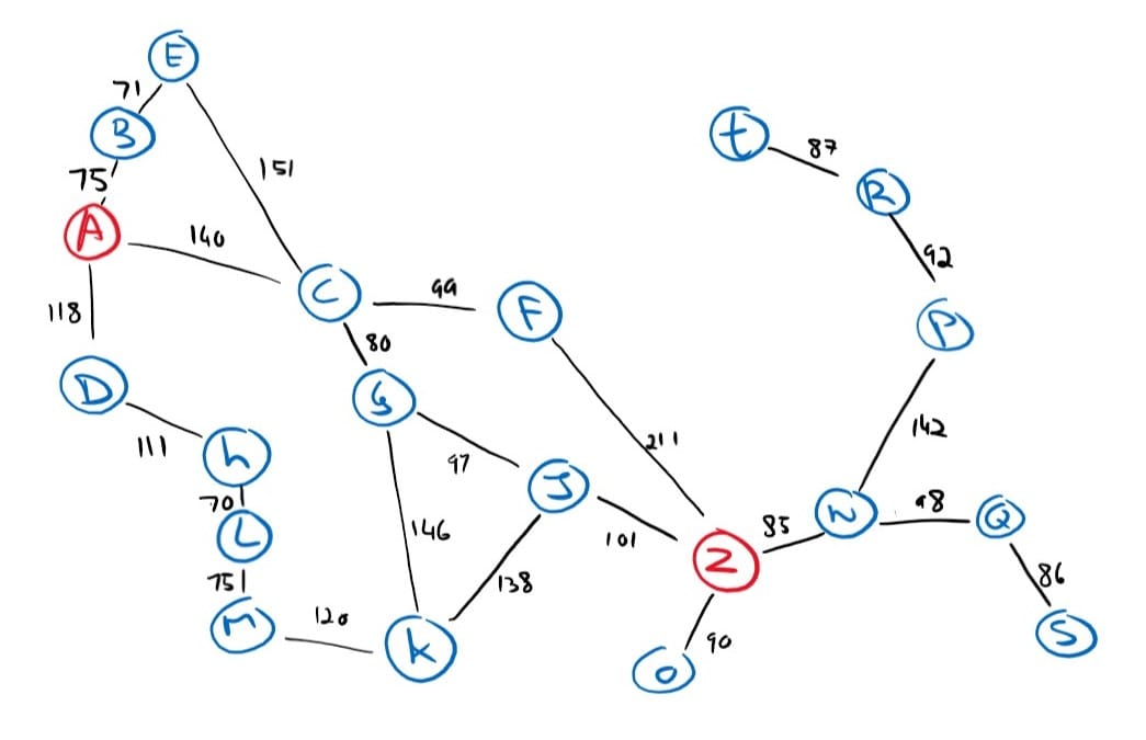
Imagine that you have the following map of your local surroundings and that you need to build an agent that will find a path from your current location A to your goal destination Z.
Before we continue, we will formally define the problem to make our lives easier by defining:
- The state space: A set of all possible states that the environment can be in.
- The initial state: The initial state that the environment starts in (the “root” of the tree).
- The goal state: A set of goal states or one goal state.
- The actions: All the actions available to the agent. Given a state s, Actions(s) returns a finite set of actions that can be executed.
- The transition model: A transition model which describes what each action does. Result(s, a) returns the state that results from doing action a in state s.
- The action cost function: A function that takes in a state, action, and the resultant state to determine the cost of an action. This can be a measure of time, resources, or work.
State space = { A, B, C, D, E, F, G, H, I, J, K, L, M, N, O, P, Q, R, S, T, Z }
Initial state = A
Goal state = Z
actions = {
    Actions(A) = { go_to_B, go_to_C, go_to_D }
    Actions(B) = { go_to_A, go_to_E }
    Actions(C) = { go_to_A, go_to_E, go_to_G, go_to_F }
    Actions(D) = { go_to_A, go_to_H }
    Actions(E) = { go_to_B, go_to_C }
    [ … ]
}
transition model = {
    Result(A, go_to_B) = B
    Result(A, go_to_C) = C
    Result(A, go_to_D) = D
    Result(B, go_to_A) = A
    Result(B, go_to_E) = E
    [ … ]
}
action cost function = {
    ActionCost(A, go_to_B, B) = 75
    ActionCost(A, go_to_C, C) = 140
    ActionCost(A, go_to_D, D) = 118
    ActionCost(B, go_to_A, A) = 75
    ActionCost(B, go_to_E, E) = 71
    [ … ]
}
And we will define an abstract Problem class as such:
class Problem(object):
   """
   An abstract search problem with core functionality that needs to be
   implemented.
   """

   def __init__(self, initial_state):
      self.initial_state = initial_state

   def actions(self, state):
      """
      Generate a list of actions that can be taken given any state.

      :param state: Any: Same datatype as the `state` in `Node`
      :return: list
      """
      raise NotImplemented("Abstract class method not implemented")

   def is_goal(self, state):
      """
      Test the given state to see if a goal has been reached. The `state` is
      of the same data type as the state in `Node` from `search_problem.util`

      :param state: Any: Same datatype as the `state` in `Node`
      :return: bool
      """
      raise NotImplemented("Abstract class method not implemented")

   def transition(self, state, action):
      """
      Generate the resultant state given any state and a valid action.

      :param state: Any: Same datatype as the `state` in `Node`
      :param action: Any
      :return: result_state: Any: Same datatype as the `state` in `Node`
      """
      raise NotImplemented("Abstract class method not implemented")

   def expand(self, node: Node):
      """
      Expand the given node with a state, return a list of successor nodes
      using the problem's actions and transitions.

      :param node: Node
      :return: list[Node]
      """
      return [Node(self.transition(node.state, action), node, action) for action in
              self.actions(node.state)]
Recall that our objective is to find a path from A to Z where each letter is a fictional city or town. A solution is found once a path from the initial state to one of the goal states is found. And so, a path is just a sequence of actions.
By the way, you may wonder if the state space should be so abstract as to include only towns and cities. Surely we would want to include different intersections within each city or town. And the answer is: it depends.
The choice of a good abstraction involves removing as much detail as possible while retaining validity and ensuring that the abstract actions can be carried out. Too many real-world details will completely overwhelm the intelligent agent.
Search Algorithms
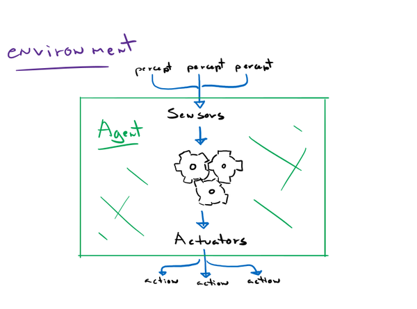
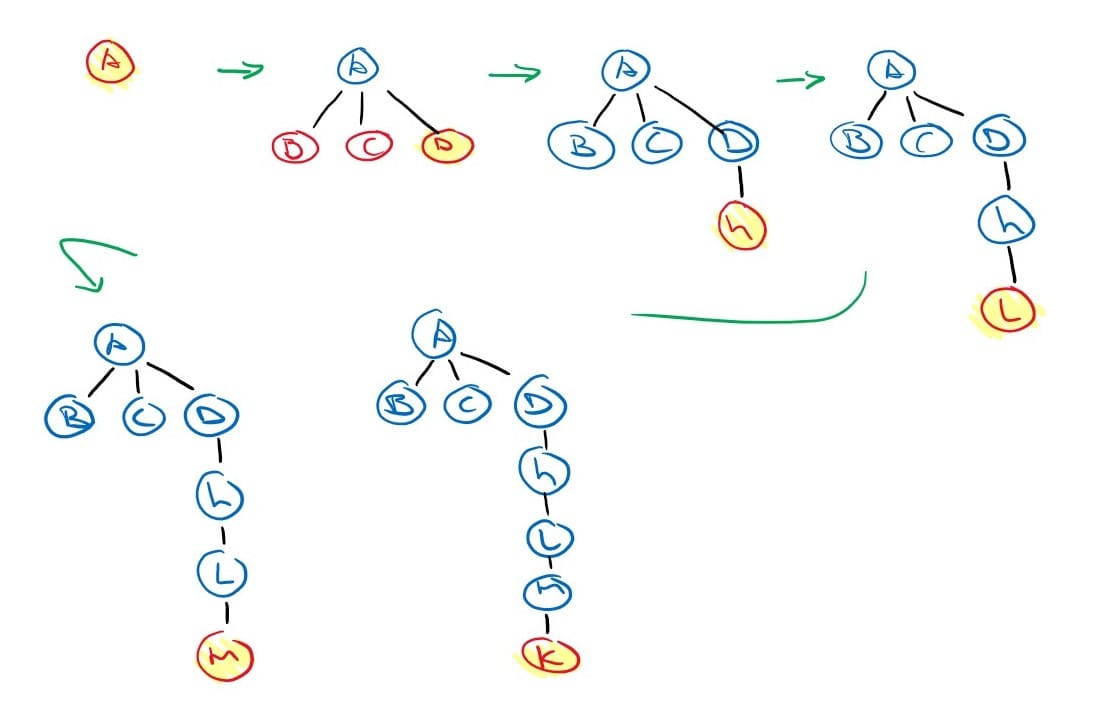
A search algorithm takes a search problem as input and returns a solution or an indication of failure. In a single-agent environment, the search algorithm will form a search tree that will superimpose the state space graph, forming various paths from the initial state, trying to find a path that reaches a goal state. Each node in the search tree corresponds to a state in the state space and the edges in the search tree correspond to actions. The root of the tree corresponds to the initial state of the problem.
It is important to understand the distinction between a state space graph and a search tree. The state space will only have as many nodes as there are states in the state space and only as many edges as there are actions, but the search tree will always have the initial state as the root node, potentially an infinite number of nodes (if we do not keep track of repeated states or cycles), but most importantly, each node in the search tree has a unique path back to the root.
The first step a search algorithm can do is expand the root node, by considering the available actions for that state through the given transition model. This will generate new nodes called successor nodes or child nodes.
Each generated node will record its parent node and will be placed in the frontier of the search tree (unexplored nodes).
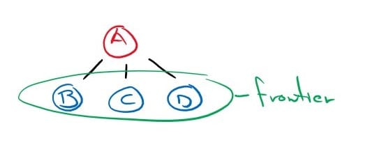
Now we must choose which of these three child nodes to consider next. This is the essence of search – following up on one option now and putting the others aside for later.
Uninformed search algorithms
An uninformed search algorithm is given no clue about how close a state is to the goal(s). It is a systematic way of exploring state space graphs and we have two strategies: breadth-first search and depth-first search.
Breadth-first Search (first-in-first-out / queue)
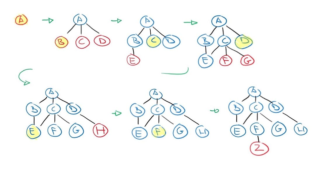
In breadth-first search, the root node is expanded first, then all its successors, and then all their successors, and so on until a goal state is found or the entire graph has been traversed.
def breadth_first_search(problem: Problem) -> Optional[Node]:
   frontier = queue.SimpleQueue()
   frontier.put(Node(problem.initial_state))

   while not frontier.empty():
      node: Node = frontier.get()
      if problem.is_goal(node.state):
         return node
      for child in problem.expand(node):
         frontier.put(child)
   return None
This strategy is implemented quite regularly because it is a complete search algorithm. Meaning that if a solution exists, this algorithm will find it. Also, it will return the solution with the fewest number of actions. And if all actions have the same cost, the solution is also a cost optimal solution.
However, this algorithm has an exponential time complexity and space complexity. Meaning that it is expensive on time and memory.
Imagine a problem where, on average, each node has ten possible actions and the solution is fifteen levels deep in the search tree.
Then we will need to generate 1 node for the root node, 10 more to expand the root node, 10 more for each of those 10 nodes, and so on 15 times. That gives us:

And if each node is allocated just a kilobyte and takes just a millisecond to process, that’s over 1000 petabytes of RAM and over 35 000 years.
We can calculate the time and space complexity more abstractly by declaring a variable ‘d’ as the depth of the solution and ‘b’ as the branching factor (average actions per node):

For this reason, this algorithm is typically not used to solve non-trivial problems.
Depth-first Search (last-in-first-out / stack)
Depth-first search algorithms will always expand the deepest node in the frontier first. Implemented with a stack (last-in-first-out). The search proceeds to expand nodes deeper and deeper until the deepest level of the search tree, where the nodes have no successors and then “backs up” to the next deepest node.
def depth_first_search(problem: Problem) -> Optional[Node]:
   frontier = queue.LifoQueue()
   frontier.put(Node(problem.initial_state))

   while not frontier.empty():
      node: Node = frontier.get()
      if problem.is_goal(node.state):
         return node
      for child in problem.expand(node):
         frontier.put(child)
   return None
This method is also complete like the breadth-first search, but it has the added benefit of reduced space complexity which comes at a cost of forgoing the optimal solutions.
The space complexity is drastically reduced from being exponentially bound to linearly bound. We now only explore one branch at a time, so our frontier includes only the successors of one node per level in the tree. Meaning that the space complexity of depth-first search is O(bm) where ‘b’ is the branching factor and ‘m’ is the maximum depth of the tree.
Cycles and Redundant Paths
We saw how both of the uninformed searches are complete, but that is only true if the state graph has no cycles. Looking at our original route-finding problem’s state graph, we can see how an algorithm can easily get stuck in an infinite loop if it were to visit A > B > E > C > A > B > E > C > A or will add redundant paths. This is especially problematic in undirected graphs like ours as each node will have an edge back to its parent; creating a duplicate sub search tree of the parent node.
We have a couple of approaches we can take to avoid redundant paths and cycles.
The first one is to remember all states we have already visited and store them in a set of ‘explored nodes’.
def breadth_first_search_with_reached(problem: Problem) -> Optional[Node]:
   explored = set()
   explored.add(problem.initial_state)
   frontier = queue.SimpleQueue()
   frontier.put(Node(problem.initial_state))

   while not frontier.empty():
      node: Node = frontier.get()
      if problem.is_goal(node.state):
         return node
      for child in problem.expand(node):
         if child.state not in explored:
            explored.add(child.state)
            frontier.put(child)
   return None
However, storing all states in memory can lead to failure just as we saw for breadth-first search algorithms. So, as a compromise, instead of holding a set of explored nodes, we can traverse the chain of parent nodes to see if a given successor node has already been explored in this particular path. This will avoid cycles, and thus infinite loops, but it can still have the same node explored multiple times from different paths.
def depth_first_search_with_reached(problem: Problem) -> Optional[Node]:
   frontier = queue.LifoQueue()
   frontier.put(Node(problem.initial_state))

   while not frontier.empty():
      node: Node = frontier.get()
      if problem.is_goal(node.state):
         return node
      for child in problem.expand(node):
         if not child.explored(child.state):
            frontier.put(child)
   return None
Depth-limited and Iterative Deepening Search
To keep depth-first search algorithms from travelling too far down a certain path. We can define a limit ‘l’ and refuse to expand nodes on that level. This allows us to not worry about infinite cycles, but of course, sometimes we may fail to find a solution if our choice of ‘l’ is too low.
def depth_limited_search(problem: Problem, depth: int) -> Optional[Node]:
   frontier = queue.LifoQueue()
   frontier.put(Node(problem.initial_state))

   while not frontier.empty():
      node: Node = frontier.get()
      if problem.is_goal(node.state):
         return node
      path = node.path_to_root()
      for child in problem.expand(node):
         if any(filter(lambda n: n.state == child.state, path)) \
            or len(path) > depth:
            # this node has either been visited or max depth reached - stop
            continue
         frontier.put(child)
   return None
This algorithm has its place in solving search problems, but it is particularly helpful when used in conjunction with an iterative deepening search algorithm.
Iterative deepening solves the problem of picking the right value of ‘l’ by trying all values sequentially from 0 to infinity.
def iterative_deepening_search(problem: Problem) -> Optional[Node]:
   for e in range(sys.maxsize):
      result = depth_limited_search(problem, e)
      if isinstance(result, Node):
         return result
Just like depth-first search and breadth-first search, iterative deepening search is complete on finite state spaces (assuming the graph is acyclic or that cycles are handled somehow), and just like breadth-first search, it will return a solution with the fewest number of actions, thus, cost optimal if all actions have the same cost. But unlike breadth-first search, it has the space complexity of depth-first search.
This essentially combines the best of both uninformed algorithms into one.
Admittedly, iterative deepening search seems wasteful at first because each call to the depth limited search will rebuild the entire search tree. But recall that the growth rate of a search tree is exponential. Meaning that each level has ‘b’ times as many nodes as the level before it. So most of the computation is in the last level anyway.
For example, take a search problem with an average branching factor of just six with a depth limit of six.
| Algorithm | Depth 0 | Depth 1 | Depth 2 | Depth 3 | Depth 4 | Depth 5 | Depth 6 | Total |
| BFS | 1 | 6 | 36 | 216 | 1296 | 7776 | 54432 | 63763 |
| DLS(0) | 1 | 1 | ||||||
| DLS(1) | 1 | 6 | 7 | |||||
| DLS(2) | 1 | 6 | 36 | 43 | ||||
| DLS(3) | 1 | 6 | 36 | 216 | 259 | |||
| DLS(4) | 1 | 6 | 36 | 216 | 1296 | 1555 | ||
| DLS(5) | 1 | 6 | 36 | 216 | 1296 | 7776 | 9331 | |
| DLS(6) | 1 | 6 | 36 | 216 | 1296 | 7776 | 54432 | 63763 |
| IDS(6) | 7 | 36 | 180 | 864 | 3888 | 15552 | 54432 | 74959 |
Looking at the table, we can see that in the worst case, breadth-first search generates 63763 nodes and iterative deepening generates 74959 nodes. Not bad, right?
Note that the difference is even smaller with a larger branching factor. In real-world problems, such as chess, branching factors can easily reach 20+.
Concrete Implementation of a Search Problem
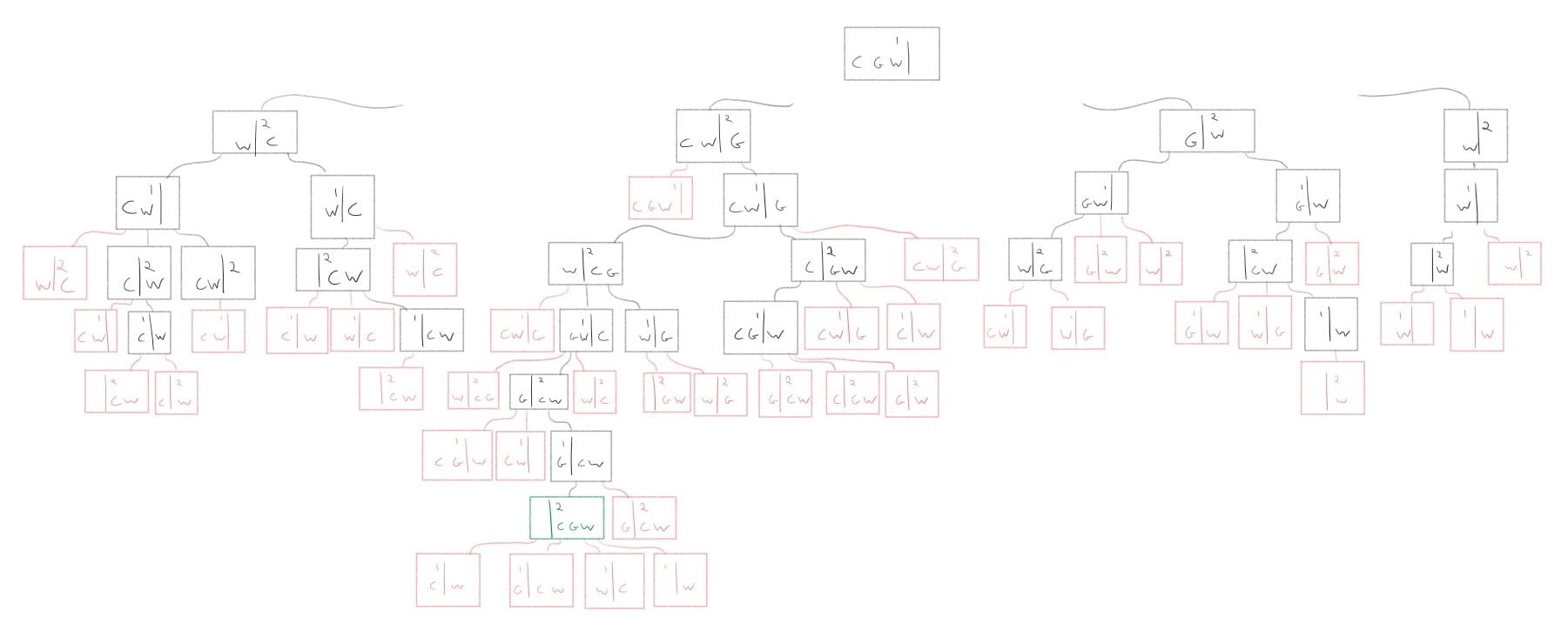
As an example, we will implement a “cabbage, goat, and wolf” problem which involves a person, travelling with a wolf, a goat and a cabbage that finds himself at a river. There is a single small boat to afford
passage across the river. The boat can hold the person and only one of the wolf, goat or cabbage. The person must ferry his animals and vegetables across the river making as many trips as necessary to do so. However, if the goat is left unattended with the cabbage, the goat will eat the cabbage. Similarly, if the wolf is left unattended with the goat, the wolf will eat the goat. How can the person ferry all items across the river without anything being eaten?
The search tree:
Implementation:
class CGW(Problem):
   """
   This class implements a Cabbage-Goat-Wolf problem as a sub-class of the
   search `Problem` class.

   The values of the state member variables of instances of this class are
   represented in a tuple as follows:

   (human, left, right)

   Where:
   human is an integer;
     1 = human (and boat) on left side,
     2 = human (and boat) on right side,

   left is a string containing zero to three of the characters "CGW" indicating
   which entities are on the left side of the river;

   right is a string containing zero to three of the characters "CGW"
   indicating which entities are on the right side of the river.

   The initial state of the CGW problem is (1,"CGW","").
   """

   def __init__(self, initial_state):
      """
      Initialize a CGW state member variables based on the passed arguments.
      """
      super().__init__(self.validate(initial_state))

   def actions(self, state):
      """
      Return a list of valid actions to take. Which are simply the animal that
      needs to be moved to the other side with the human.

      Recall that a state is: (human, left_side, right_side) where human is
      1 if on the left side or 2 if on the right.

      So we can access the side we are working on using:

         state[state[0]] -> state[human location] -> the side human is on

      """
      actions = []
      for animal in state[state[0]]:
         actions.append(animal)  # animal crossing with human
      actions.append(None)  # the human crossing alone

      return actions

   def is_goal(self, state):
      """
       Return True if the problem is solved.  I.e.: human and all items are on
       the right side.
       """
      return state[0] == 2 and state[2] == "CGW"

   def transition(self, state, action):
      """
      The transition is to always move the human from one side to the other.
      The action contains a letter "C", "G", "W" to indicate which animal
      should the human take with him, or `None` if the human is to move alone.
      """
      animal = action
      human = state[0]
      left_side = state[1]
      right_side = state[2]

      if human == 1:
         # human is going from left to right, move animal from left to right
         human = 2
         left_side = self._remove_animal(left_side, animal)
         right_side = self._add_animal(right_side, animal)

      elif human == 2:
         human = 1
         # human is going from right to left, move animal from right to left
         right_side = self._remove_animal(right_side, animal)
         left_side = self._add_animal(left_side, animal)

      else:  # Where is the human ?
         raise IndexError("State[0] 'human' must be '1' or '2'.")

      state = (human, left_side, right_side)
      return self.validate(state)

   def validate(self, state):
      """
      Update a state variable based on the goat eating the cabbage or the wolf
      eating the goat.
      """
      if state[0] == 1:  # human is on left side
         right = state[2]  # retrieve the contents of the right side
         if "G" in right:  # goat is on right side
            right = self._remove_animal(right, "C")  # goat eats cabbage
         if "W" in right:  # wolf is on right side
            right = self._remove_animal(right, "G")  # wolf eats cabbage
         # reconstruct state which with new right-side contents
         state = (state[0], state[1], right)

      elif state[0] == 2:  # human is on right side
         left = state[1]  # retrieve the contents of the left side
         if "G" in left:  # goat is on the left side
            left = self._remove_animal(left, "C")  # goat eats cabbage
         if "W" in left:  # wolf is on the left side
            left = self._remove_animal(left, "G")  # wolf eats goat
         # reconstruct state with new left-side contents
         state = (state[0], left, state[2])

      else:  # Where is the human ?
         raise IndexError("State[0] 'human' must be '1' or '2'.")
      return state

   def _remove_animal(self, input_string, animal):
      """
      This is a utility function that returns a string that matches the
      input_string except with the given animal (letter) removed.

      exp: input: "CGW", animal: "G", output: "CW"
      """
      if animal is None:
         return input_string
      return input_string.replace(animal, "")

   def _add_animal(self, input_string, animal):
      """
      This is a utility function that returns a string that matches the
      input_string with the given animal added in alphabetical position.
      """
      if animal is None:
         return input_string
      return "".join(sorted(input_string + animal))
initial_state = (1, "CGW", "")
node = iterative_deepening_search(CGW(initial_state))
if node is not None:
solution = node.solution()
for index, action in enumerate(solution):
if action is None:
solution[index] = '-'
print("".join(solution))
else:
print("No solution found")Run:
> G-WGC-G