Heuristic Search Algorithms

In the last article, we saw how a problem-solving agent could use search trees to look ahead and find a sequence of actions that will solve a problem, but we faced a drastic issue: uninformed search trees grow too fast!
This article will see how we can pick more promising paths first and put aside the least likely ones for last, known as a best-first search or uniform-cost search. The idea is that while breadth-first search spreads out in waves of uniform depths (depth 1 -> depth 2 -> … ), best-first search spreads out in waves of uniform evaluations ( f(n) ).
Best-first Search
A very general approach in which we choose a node, n, with minimum values of some evaluation function, f(n). On each iteration, we choose a node on the frontier with a minimum f(n) value, return it if its state is a goal state, and otherwise expand it to generate child nodes. Each child node is added to the frontier if it has not been reached before or is re-added if reached from a less costly path. By employing different evaluation functions, we get different specific algorithms, which we discuss in this article.
def best_first_search(problem: Problem, f: Callable) -> Optional[Node]:
   """
   Takes in an implemented `Problem` and returns a `Node` once a solution is
   found or `None` otherwise. Uses a priority queue to always explore nodes
   in the frontier with the lowest f(n) value.

   This algorithm will track reached/explored nodes and will insert a node into
   the frontier if that node has not been reached before, or if the new path has
   a lower cost. To avoid duplicates in the frontier, use an A* search with a
   monotonic heuristic.

   :param problem: Implemented Problem class
   :param f: Callable evaluation function that takes in 1 argument; Node
   :return: Node or None
   """
   explored = {}
   frontier = []

   root = Node(problem.initial_state)
   counter = itertools.count()  # tie breaker for heapq
   heapq.heappush(frontier, (f(root), next(counter), root))

   while frontier:
      node: Node = heapq.heappop(frontier)[2]
      if problem.is_goal(node.state):
         return node
      for child in problem.expand(node):
         if child.state in explored \
            and f(child) >= explored[child.state].path_cost:
            continue
         heapq.heappush(frontier, (f(child), next(counter), child))
         explored[node.state] = child
   return None
Heuristic Function
A heuristic function will take a node and evaluate how close it is to the solution. It uses domain-specific clues to estimate the cheapest path from the given node to a goal. We typically want heuristics that underestimate the actual cost ( optimistic heuristic ) rather than overestimating ( pessimistic heuristic ). If the heuristic is too high, then we don’t explore nodes, and we might miss a low-cost solution, but if the estimate is too low, then we tend to expand nodes and then later discard them when the actual cost for the node starts adding up.
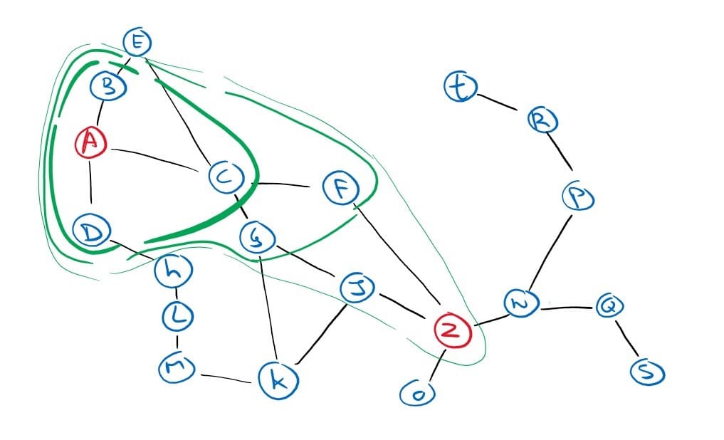
Recall our fictional map of towns from the last article, for which we will create an example of an optimistic heuristic function.
Our heuristic will return the straight line distance between any node and the goal from that map. And we use that distance as an estimate to evaluate a node. It is optimistic because a straight line between two points will always be less than or equal to any other path.

Greedy Best-first Search
A greedy best-first search is a form of best-first search that expands the node with the lowest heuristic value or, in other words, the node that appears to be the most promising. And recall that a best-first search algorithm will pick the node with the lowest evaluation function. So, a greedy best-first search is a best-first search where f(n) = h(n).
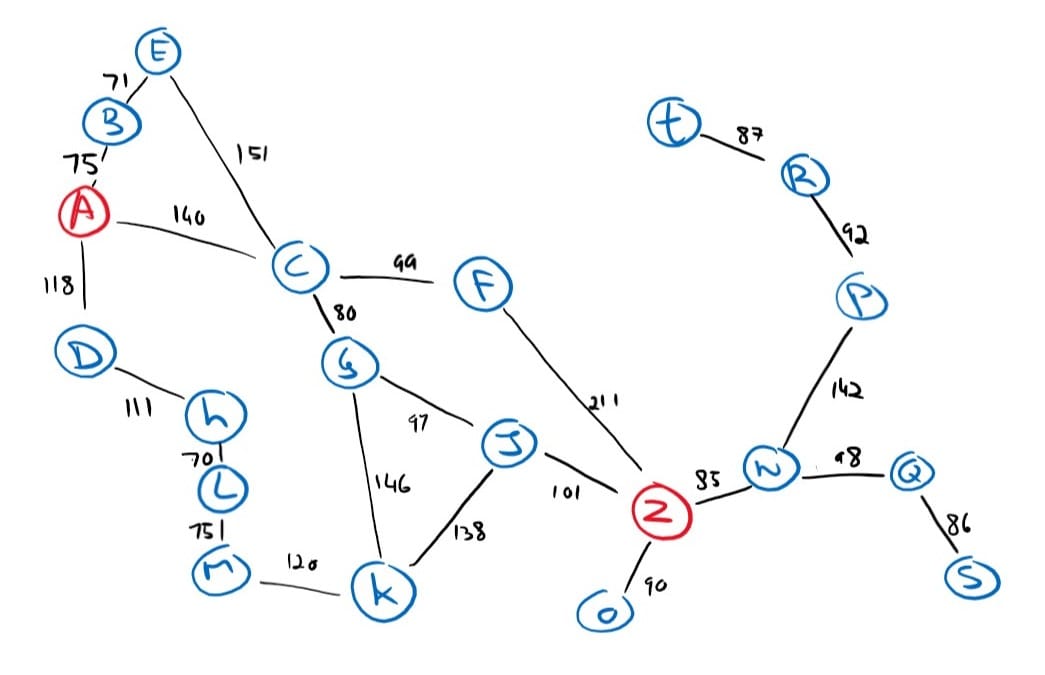
As an example, we will look for a path from A to Z using the greedy approach.
Our heuristic values:
| h(A) = 366 | h(E) = 380 | h(J) = 100 | h(N) = 80 | h(R) = 226 |
| h(B) = 374 | h(F) = 176 | h(K) = 160 | h(O) = 77 | h(S) = 161 |
| h(C) = 253 | h(G) = 193 | h(L) = 241 | h(P) = 199 | h(T) = 234 |
| h(D) = 329 | h(H) = 244 | h(M) = 242 | h(Q) = 151 | h(Z) = 0 |
The algorithm will create a search tree internally, just like uninformed searches. Still, I find it easier to superimpose the search tree onto the state graph to demonstrate better how the frontier is expanded closer and closer toward the goal.
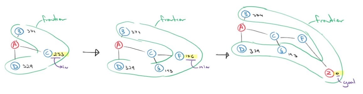
We first expand our initial node A, and we get three successor nodes; B, C and D. Looking at our heuristic values table, we determine that C is the closest to the goal, so we expand it and add its successors to the frontier. We continue to do so until we reach the goal. Notice that the algorithm did not expand a single node that is not on the path to the solution. However, the solution found is not the optimal solution. The optimal path is ‘go_to_C’, ‘go_to_G’, ‘go_to_J’, ‘go_to_Z’, but our algorithm did not find it. Greedy best-first search is not concerned with the cost already incurred nor the cost to reach a promising node. It just expands the most promising node from the frontier, and this is why it’s called a greedy approach.
When using this approach, we keep track of all visited nodes, and so, space and time complexity is equal to the size of the state space. And, assuming that the state space is finite, greedy search is a complete search algorithm.
A* search
A more common approach to solving search problems is the A-star search, which is a best-first search that employs the heuristic function as well, but unlike greedy best-first search, A-star search will include the cost incurred to reach a node in conjunction with the heuristic value. And so, its evaluation function is f(n) = g(n) + h(n) where g(n) is the cost to reach a node n from the initial state and h(n) is the heuristic value of that same node.
In other words, the evaluation function returns the exact cost to reach node n plus an estimate of the cost remaining to reach the goal from node n.
We will do another example using the same heuristic table and search problem as we did for the greedy best-first search, but this time using A* search.
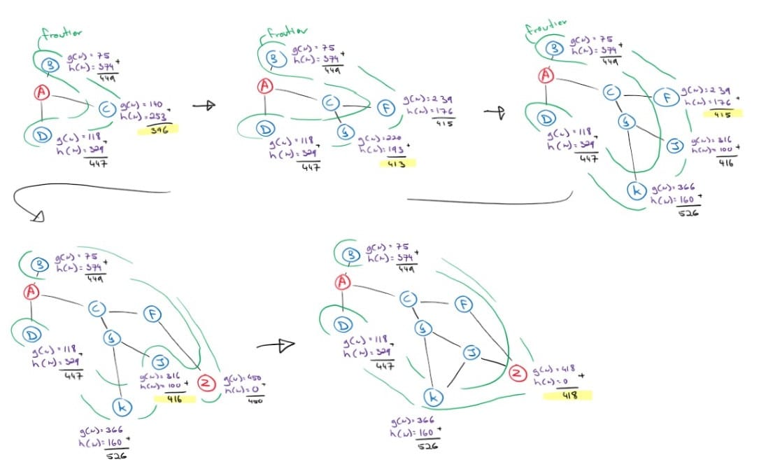
There are a few things to note here. Contrary to the greedy search, A-star’s frontier expands conservatively yet steadily towards the goal. Also, notice that we had to explore more nodes to find a solution because A* search is careful. It also perceived the less optimal solution when it expanded node F (4th graph) with an f(n) value of 450, but another node, J, saw a possible path to the goal with an f(n) value of 416. And so, the algorithm explored node J before returning a solution that it had already found. Sure enough, the path through J found another, better solution. In fact, it’s the cost-optimal solution.
Whether A* is cost-optimal depends entirely on two properties of the heuristic function selected. It needs to be admissible and monotonic.
Admissibility
An admissible heuristic is one that never overestimates the cost to reach a goal. And as long as your heuristic is admissible, you will get a cost-optimal solution. The intuition behind it is that an admissible heuristic will always return the minimum cost, and at the very least, you will need to spend g(n) + h(n) to go down path n. If you found a solution that costs less than all the evaluation values in the frontier, you are guaranteed to have found the optimal solution. This can be shown more formally through a proof by contradiction.
Suppose an optimal solution exists with a cost C*, but our algorithm returned another solution with a cost C, greater than C*. Then that means a node n that is on the optimal path has not been expanded. And because we are using a best-first search algorithm, it must mean that the evaluation value of that node was greater than C, and thus, greater than C* (otherwise, we would have expanded it). For this proof, we denote c(n, z) as the optimal cost from node n to the goal.

by A* definition, we get

because h(n) is admissible, we get

because n is on the optimal path, the cost to reach n in conjunction with the optimal cost to reach the goal from n, we get the optimal cost, C*.

The first and last lines form a contradiction, so it is not possible to have a node on the optimal path unexplored, and thus, impossible to return a suboptimal solution.
Monotonicity
A stronger property of a heuristic function is monotonicity or sometimes called consistency. A heuristic is monotonic if the evaluation function is monotonically increasing as we explore a path. Or in other words, it means that if my heuristic evaluates a node at a particular value, not only will it be an optimistic estimate, but it is also the minimum cost to pursue a solution through that node.
More formally, we have:

Where n is any node and n’ is any of its successors. This inequality must hold for every node, so it’s true for its successors n’ as well. And so we have:

And from here, you can see a pattern. Once h(n) is evaluated, it can only increase or stay the same. Hence the name monotonic.
Admissible vs monotonic
Every monotonic heuristic is admissible, but not every admissible heuristic is monotonic. And so, just like an admissible heuristic, a monotonic heuristic will return a cost-optimal solution. But in addition, with a monotonic heuristic, the first time we reach a node, it will be on an optimal path, so we never have to re-add a node to the frontier.
If it cannot be shown that a heuristic is monotonically increasing, then we cannot guarantee that every node in the frontier has the lowest evaluation value. We may reach a node in the frontier from a different path with a lower cost. Suppose a heuristic is admissible but not monotonic. In that case, we have to keep track of all the nodes in the frontier and update their values, parent and successors when we find a better path, or we must introduce duplicate nodes in our frontier. For this reason, it’s best to use a monotonic heuristic if possible.
Inadmissible heuristics
As powerful as an A* search can be, it can sometimes have a high space and time complexity. An admissible heuristic cannot take risks because it needs to guarantee a minimal cost. This restriction can return conservative heuristic values and rank all successors equally. In such a case, an A* search can turn into a breadth-first search. But if we are willing to accept the possibility of a suboptimal solution, we may use an inadmissible heuristic. A heuristic that may overestimate the cost but does a much better job of estimating a solution’s cost.
Inventing heuristic functions
Sometimes inventing a good heuristic can be challenging, so I want to pass along a helpful tip before I end this article. Take an 8-puzzle problem as an example.
For those not familiar with an 8-puzzle problem, the premise is simple. You are presented with a board that can fit nine tiles, but only eight are present. You must rearrange the tiles until the numbers are sorted, like in the goal image below.
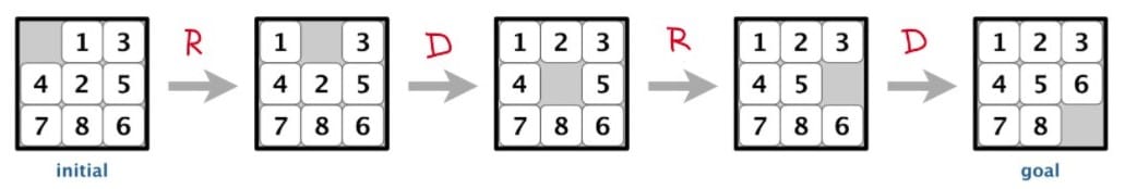
There is only one rule:
You can move tile X to position Y if Y is adjacent to X and if Y is empty.
A concrete implementation of an 8-Puzzle problem
class Puzzle(Problem):
   """
   The values of the state member variables of instances of this class are
   represented as a string as follows:

   "12345678_" where '_' represents the empty tile.

   The inital state of the Puzzle problem is completely random.
   """

   def actions(self, state):
      """
      Actions labeled with 'U', 'D', 'L' or 'R' indicate the direction taken
      by the blank space.

      eg: +-------+      +-------+
         | _ 2 3 |      | 1 2 3 |
         | 1 4 6 | -D-> | _ 4 6 |
         | 7 5 8 |      | 7 5 8 |
         +-------+      +-------+
      """
      actions = []
      index = state.index('_')
      if int(index / 3) > 0:
         # "move up allowed"
         actions.append('U')

      if int(index / 3) < 2:
         # "move down allowed"
         actions.append('D')

      if index % 3 > 0:
         # "move left allowed"
         actions.append('L')

      if index % 3 < 2:
         # "move right allowed"
         actions.append('R')

      return actions

   def is_goal(self, state):
      """
      Return True if the problem is solved.  I.e.: human and all items are on
      the right side.
      """
      return state == '12345678_'

   def transition(self, state, action):
      """
      Paths labeled with 'U', 'D', 'L' or 'R' indicate the direction taken by the
      blank space.

      eg: +-------+      +-------+
         | _ 2 3 |      | 1 2 3 |
         | 1 4 6 | -D-> | _ 4 6 |
         | 7 5 8 |      | 7 5 8 |
         +-------+      +-------+
      """
      index = state.index('_')
      if action == 'U':
         # "move up"
         new_state = list(state)
         new_state[index - 3], new_state[index] = new_state[index], new_state[index - 3]
         return ''.join(new_state)

      if action == 'D':
         # "move down"
         new_state = list(state)
         new_state[index + 3], new_state[index] = new_state[index], new_state[index + 3]
         return ''.join(new_state)

      if action == 'L':
         # "move left"
         new_state = list(state)
         new_state[index - 1], new_state[index] = new_state[index], new_state[index - 1]
         return ''.join(new_state)

      if action == 'R':
         # "move right"
         new_state = list(state)
         new_state[index + 1], new_state[index] = new_state[index], new_state[index + 1]
         return ''.join(new_state)
One method to create a heuristic for this problem is to use what’s known as a relaxed problem approach. We relax the restrictions and open more edges between nodes in the state graph. The added edges will simplify the computation needed to find a solution, and we use the solution to the simplified problem as a heuristic to our original problem. Because we are exploring the same state graph but with more paths, we are guaranteed to find an optimistic solution. For example, with the 8-puzzle problem, we can remove the restriction that Y must be adjacent to X and Y must be empty. The relaxed problem becomes:
You can move tile X to position Y if Y is adjacent to X and if Y is empty.
This heuristic is called the ‘misplaced tiles’ heuristic. It will always underestimate the true cost because it is synonymous with you just lifting a tile and placing it where it belongs. For each tile that isn’t where it is supposed to be, it will cost you at least one action to move it.
Or, we can remove the restriction that Y must be empty, and we get:
You can move tile X to position Y if Y is adjacent to X and if Y is empty.
The result is a heuristic that measures the sum of the distances of the tiles from their goal positions. Because this heuristic has more restrictions than the misplaced tiles heuristic, it is better at estimating the true cost, and thus, will find a solution quicker. But because it has fewer restrictions than the original problem, it is still an admissible heuristic.
Solving an 8-puzzle using a misplaced tiles heuristic:
def misplaced_tiles_heuristic(node: Node) -> int:
   """
   Return the heuristic value of a given node. The heuristic will count how
   many tiles are not in their designated position which indicates a minimum
   number of moves needed to solve the problem.

   :param node: Node
   :return: int
   """
   heuristic = -1
   for (e, i) in zip(node.state, '12345678*'):
      heuristic += int(e == i)
   return heuristic
Solution:
initial_state = '_13425786'
print('Initial State:')
print_puzzle(initial_state)
problem = Puzzle(initial_state)

node = a_star_search(problem, misplaced_tiles_heuristic)
if node is not None:
   solution = node.solution()
   print("Solution:", "".join(solution))
else:
   print("No solution found")
Initial State:
+-------+
| _ 1 3 |
| 4 2 5 |
| 7 8 6 |
+-------+
Solution: RDRD